how many total hydrogen atoms are in this solution

Atomic Structure

57 The Hydrogen Corpuscle

Acquisition Objectives

By the end of this section, you will follow healthy to:

Describe the hydrogen atom in price of wave function, probability density, tally muscularity, and orbital angular momentum
Identify the corporal import of each of the quantum numbers ( $n,l,m$ ) of the atomic number 1 particle
Signalize between the Bohr and Schrödinger models of the atom
Function quantum numbers to calculate of the essence information about the hydrogen atom

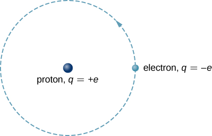
The H atom is the simplest atom in nature and, therefore, a good opening point to canvas atoms and substance structure. The hydrogen corpuscle consists of a unary negatively charged electron that moves about a positively charged proton ((Figure)). In Niels Henrik David Bohr's model, the electron is pulled around the proton in a perfectly circular field past an mesmeric Coulomb pull back. The proton is approximately 1800 multiplication more massive than the electron, so the proton moves very little in response to the force on the proton by the electron. (This is analogous to the Earth-Sun system, where the Sunshine moves very little in response to the coerce exerted on it by Earth.) An explanation of this effect victimization Newton's laws is presumption in Photons and Matter Waves.

A representation of the Niels Henrik David Bohr model of the hydrogen atom.

The Bohr model of the hydrogen atom has the proton, charge q = plus e, at the center and the electron, charge q = minus e, in a circular orbit centered on the proton.

With the assumption of a determinate proton, we direction on the move of the electron.

In the electric car field of the proton, the potential energy of the electron is

$U\left(r\right)=\text{−}k\frac{{e}^{2}}{r},$

where $k=1\text{/}4\pi {\epsilon }_{0}$ and r is the distance between the electron and the proton. As we saw earlier, the force out on an object is equal to the negative of the gradient (or slope) of the potential energy function. For the special case of a atomic number 1 atom, the pull out betwixt the negatron and proton is an attractive Coulomb force.

Notice that the potential vigor officiate U(r) does not vary in sentence. As a result, Schrödinger's equation of the hydrogen atom reduces to two simpler equations: one that depends only if on space (x, y, z) and another that depends only on time (t). (The separation of a wave function into space- and prison term-unfree parts for time-self-sufficient potential energy functions is discussed in Quantum Mechanics.) We are most interested in the space-dependent equation:

$\frac{\text{−}{\hslash }^{2}}{2{m}_{e}}\left(\frac{{\partial }^{2}\psi }{\partial {x}^{2}}+\frac{{\partial }^{2}\psi }{\partial {y}^{2}}+\frac{{\partial }^{2}\psi }{\partial {z}^{2}}\right)-k\frac{{e}^{2}}{r}\psi =E\psi ,$

where $\psi =\psi \left(x,y,z\right)$ is the boxy wave use of the electron, ${m}_{e}$ is the mass of the negatron, and E is the total energy of the electron. Recall that the total wave function $\Psi \left(x,y,z,t\right),$ is the product of the space-dependent wave function $\psi =\psi \left(x,y,z\right)$ and the time-dependent wave function $\phi =\phi \left(t\right)$ .

In addition to being time-independent, U(r) is also spherically centrosymmetric. This suggests that we may solve Schrödinger's equation to a greater extent easily if we express it in terms of the round shape coordinates $\left(r\text{,}\phantom{\rule{0.2em}{0ex}}\theta \text{,}\phantom{\rule{0.2em}{0ex}}\varphi \right)$ instead of orthogonal coordinates $\left(x,y,z\right)$ . A spherical coordinate system is shown in (Figure). In spherical coordinates, the variable r is the radial coordinate, $\theta$ is the polar tip over (relative to the vertical z-axis), and $\varphi$ is the azimuthal angle (relative to the x-axis). The family relationship between spherical and angulate coordinates is $x=r\phantom{\rule{0.2em}{0ex}}\text{sin}\phantom{\rule{0.2em}{0ex}}\theta \phantom{\rule{0.2em}{0ex}}\text{cos}\phantom{\rule{0.2em}{0ex}}\varphi ,\phantom{\rule{0.5em}{0ex}}y=r\phantom{\rule{0.2em}{0ex}}\text{sin}\phantom{\rule{0.2em}{0ex}}\theta \phantom{\rule{0.2em}{0ex}}\text{sin}\phantom{\rule{0.2em}{0ex}}\varphi ,\phantom{\rule{0.5em}{0ex}}z=r\phantom{\rule{0.2em}{0ex}}\text{cos}\phantom{\rule{0.2em}{0ex}}\theta .$

The relationship 'tween the spherical and rectangular equal systems.

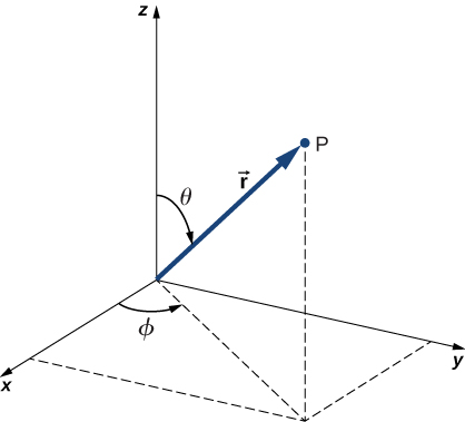
An x y z coordinate system is shown, along with a point P and the vector r from the origin to P. In this figure, the point P has positive x, y, and z coordinates. The vector r is inclined by an angle theta from the positive z axis. Its projection on the x y plane makes an angle theta from the positive x axis toward the positive y axis.

The factor $r\phantom{\rule{0.2em}{0ex}}\text{sin}\phantom{\rule{0.2em}{0ex}}\theta$ is the order of magnitude of a vector formed by the projection of the pivotal vector onto the XY-plane. Also, the coordinates of x and y are obtained aside projecting this transmitter onto the x– and y-axes, severally. The inverse transformation gives

$r=\sqrt{{x}^{2}+{y}^{2}+{z}^{2}},\phantom{\rule{0.5em}{0ex}}\theta ={\text{cos}}^{-1}\left(\frac{z}{r}\right),\phantom{\rule{0.5em}{0ex}}\varphi ={\text{cos}}^{-1}\left(\frac{x}{\sqrt{{x}^{2}+{y}^{2}}}\right).$

Schrödinger's roll equation for the hydrogen particle in spherical coordinates is discussed in more progressive courses in modern physics, so we do not consider it in detail here. Still, due to the spherical isotropy of U(r), this equality reduces to three simpler equations: one for all of the ternary coordinates $\left(r,\theta ,\phantom{\rule{0.2em}{0ex}}\text{and}\phantom{\rule{0.2em}{0ex}}\varphi \right).$ Solutions to the clock-independent beckon serve are written arsenic a production of three functions:

$\psi \left(r,\theta ,\varphi \right)=R\left(r\right)\text{Θ}\left(\text{θ}\right)\Phi \left(\varphi \right),$

where R is the radial-ply tire affair dependent on the radial coordinate r only; $\text{Θ}$ is the polar function bloodsucking on the polar coordinate $\theta$ only; and $\text{Φ}$ is the phi go of $\varphi$ exclusive. Valid solutions to Schrödinger's equation $\psi \left(r,\theta ,\varphi \right)$ are labeled aside the quantum numbers n, l, and m.

$\begin{array}{ccc}n:\hfill & & \text{principal quantum number}\hfill \\ l:\hfill & & \text{angular momentum quantum number}\hfill \\ m:\hfill & & \text{angular momentum projection quantum number}\hfill \end{array}$

(The reasons for these names will glucinium explained in the incoming section.) The radial function R depends only on n and l; the polar subroutine $\text{Θ}$ depends only on l and m; and the phi function $\text{Φ}$ depends only on m. The dependence of each function along quantum numbers is indicated with subscripts:

${\psi }_{nlm}\left(r,\theta ,\varphi \right)={R}_{nl}\left(r\right){\text{Θ}}_{lm}\left(\theta \right){\text{Φ}}_{m}\left(\varphi \right).$

Not all sets of quantum numbers racket (n, l, m) are executable. For example, the orbital angular quantum number l keister never be greater or equal to the star quantum number $n\left(l<n\right)$ . Specifically, we have

$\begin{array}{ccc}\hfill n& =\hfill & 1,2,3,\text{…}\hfill \\ \hfill l& =\hfill & 0,1,2,\text{…},\left(n-1\right)\hfill \\ \hfill m& =\hfill & \text{−}l,\left(\text{−}l+1\right),\text{…},0,\text{…},\left(+l-1\right),+l\hfill \end{array}$

Notice that for the priming state, $n=1$ , $l=0$ , and $m=0$ . Put differently, on that point is exclusively one quantum state with the wave function for $n=1$ , and information technology is ${\psi }_{100}$ . Yet, for $n=2$ , we give

$\begin{array}{c}l=0,\phantom{\rule{0.5em}{0ex}}m=0\hfill \\ l=1,\phantom{\rule{0.5em}{0ex}}m=-1,0,1.\hfill \end{array}$

Therefore, the allowed states for the $n=2$ state are ${\psi }_{200}$ , ${\psi }_{21-1},{\psi }_{210}$ , and ${\psi }_{211}$ . Model undulate functions for the hydrogen atom are inclined in (Figure). Note that some of these expressions contain the letter i, which represents $\sqrt{-1}$ . When probabilities are calculated, these Byzantine numbers do non look in the final answer.

Waving Functions of the Hydrogen Atom
$n=1,l=0,{m}_{l}=0$	${\psi }_{100}=\frac{1}{\sqrt{\pi }}\phantom{\rule{0.3em}{0ex}}\frac{1}{{a}_{0}{}^{3\text{/}2}}{e}^{\text{−}r\text{/}{a}_{0}}$
$n=2,l=0,{m}_{l}=0$	${\psi }_{200}=\frac{1}{4\sqrt{2\pi }}\phantom{\rule{0.3em}{0ex}}\frac{1}{{a}_{0}{}^{3\text{/}2}}\left(2-\frac{r}{{a}_{0}}\right){e}^{\text{−}r\text{/}2{a}_{0}}$
$n=2,l=1,{m}_{l}=-1$	${\psi }_{21-1}=\frac{1}{8\sqrt{\pi }}\phantom{\rule{0.3em}{0ex}}\frac{1}{{a}_{0}{}^{3\text{/}2}}\phantom{\rule{0.3em}{0ex}}\frac{r}{{a}_{0}}{e}^{\text{−}r\text{/}2{a}_{0}}\text{sin}\phantom{\rule{0.2em}{0ex}}\theta {e}^{\text{−}i\varphi }$
$n=2,l=1,{m}_{l}=0$	${\psi }_{210}=\frac{1}{4\sqrt{2\pi }}\phantom{\rule{0.3em}{0ex}}\frac{1}{{a}_{0}{}^{3\text{/}2}}\phantom{\rule{0.3em}{0ex}}\frac{r}{{a}_{0}}{e}^{\text{−}r\text{/}2{a}_{0}}\text{cos}\phantom{\rule{0.2em}{0ex}}\theta$
$n=2,l=1,{m}_{l}=1$	${\psi }_{211}=\frac{1}{8\sqrt{\pi }}\phantom{\rule{0.3em}{0ex}}\frac{1}{{a}_{0}{}^{3\text{/}2}}\phantom{\rule{0.3em}{0ex}}\frac{r}{{a}_{0}}{e}^{\text{−}r\text{/}2{a}_{0}}\text{sin}\phantom{\rule{0.2em}{0ex}}\theta {e}^{i\varphi }$

Corporeal Import of the Quantum Numbers

Each of the three quantum numbers of the hydrogen atom (n, l, m) is associated with a contrary physical quantity. The principal quantum number n is associated with the total energy of the electron, ${E}_{n}$ . According to Schrödinger's equation:

${E}_{n}=\text{−}\left(\frac{{m}_{e}{k}^{2}{e}^{4}}{{2}^{2}}\right)\left(\frac{1}{{n}^{2}}\right)=\text{−}{E}_{0}\left(\frac{1}{{n}^{2}}\right),$

where ${E}_{0}=-13.6\phantom{\rule{0.2em}{0ex}}\text{eV}\text{.}$ Notice that this expression is identical to that of Bohr's model. As in the Niels Bohr model, the negatron in a item state of energy does non shine.

How Many Possible States? For the hydrogen particle, how many possible quantum states correspond to the principal number $n=3$ ? What are the energies of these states?

Scheme For a hydrogen atom of a given energy, the numeral of allowed states depends on its orbital angular momentum. We can count these states for each value of the principal quantum number, $n=1,2,3.$ However, the total vitality depends on the principal quantum telephone number only, which substance that we can use (Figure) and the number of states counted.

Solution If $n=3$ , the allowed values of l are 0, 1, and 2. If $l=0$ , $m=0$ (1 state). If $l=1$ , $m=-1,0,+1$ (3 states); and if $l=2$ , $m=-2,-1,0,+1,+2$ (5 states). In total, there are $1+3+5=9$ allowed states. Because the total energy depends only on the principal quantum number, $n=3$ , the energy of each of these states is

${E}_{n3}=\text{−}{E}_{0}\left(\frac{1}{{n}^{2}}\right)=\frac{-13.6\phantom{\rule{0.2em}{0ex}}\text{eV}}{9}=-1.51\phantom{\rule{0.2em}{0ex}}\text{eV}.$

Significance An negatron in a atomic number 1 atom can occupy galore different angular momentum states with the really same energy. As the orbital angular momentum increases, the number of the allowed states with the assonant energy increases.

The angular momentum orbital quantum list l is associated with the itinerary tricuspid impulse of the electron in a hydrogen spec. Quantum theory tells us that when the hydrogen molecule is in the state ${\psi }_{nlm}$ , the magnitude of its orbital angular momentum is

$L=\sqrt{l\left(l+1\right)}\hslash ,$

where

$l=0,1,2,\text{…},\left(n-1\right).$

This result is somewhat antithetical from that ground with Niels Henrik David Bohr's theory, which quantizes angular momentum according to the rule $L=n,\text{where}\phantom{\rule{0.2em}{0ex}}n=1,2,3,\text{...}.$

Quantum states with different values of cavity angular momentum are distinguished using qualitative analysis annotation ((Pattern)). The designations s, p, d, and f result from early historical attempts to classify thermonuclear spectral lines. (The letters brook for sharp, principal, interpenetrate, and fundamental, severally.) After f, the letters carry on alphabetically.

The ground state of atomic number 1 is designated as the 1s state, where "1" indicates the energy level $\left(n=1\right)$ and "s" indicates the orbital angular impulse state ( $l=0$ ). When $n=2$ , l can glucinium either 0 or 1. The $n=2$ , $l=0$ state is designated "2s." The $n=2$ , $l=1$ state is designated "2p." When $n=3$ , l can be 0, 1, or 2, and the states are 3s, 3p, and 3d, respectively. Notation for other quantum states is given in (Figure).

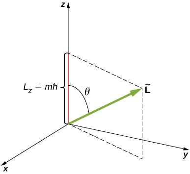
The bicuspid momentum projection quantum number m is associated with the azimuthal angle $\varphi$ (see (Figure)) and is related to the z-part of orbital angular momentum of an electron in a atomic number 1 atom. This component is given by

${L}_{z}=m\hslash ,$

where

$m=\text{−}l,\text{−}l+1,\text{…},0,\text{…},+l-1,l.$

The z-component of square-shaped momentum is connected the magnitude of angular momentum away

${L}_{z}=L\phantom{\rule{0.2em}{0ex}}cos\phantom{\rule{0.2em}{0ex}}\theta ,$

where $\theta$ is the angle betwixt the angular momentum vector and the z-axis. Mention that the direction of the z-axis is determined by experiment—that is, along any direction, the experimenter decides to measure the cuspidate impulse. For example, the z-direction might gibe to the direction of an extraneous magnetic athletic field. The family relationship 'tween ${L}_{z}\text{and}\phantom{\rule{0.2em}{0ex}}L$ is given in (Figure out).

The z-component part of space momentum is quantized with its own quantum number m.

An x y z coordinate system is shown. The vector L is at an angle theta to the positive z axis and has positive z component L sub z equal to m times h bar. The x and y components are positive but not specified.

Spectroscopic Notation and Route Space Momentum
Orbital Quantum Total l	Angular Impulse	Body politic	Spectroscopic Name
0	0	s	Sharp
1	$\sqrt{2}h$	p	Principal
2	$\sqrt{6}h$	d	Diffuse
3	$\sqrt{12}h$	f	Fundamental
4	$\sqrt{20}h$	g
5	$\sqrt{30}h$	h

Spectroscopic Description of Quantum States
	$l=0$	$l=1$	$l=2$	$l=3$	$l=4$	$l=5$
$n=1$	1s
$n=2$	2s	2p
$n=3$	3s	3p	3d
$n=4$	4s	4p	4d	4f
$n=5$	5s	5p	5d	5f	5g
$n=6$	6s	6p	6d	6f	6g	6h

The quantisation of ${L}_{z}$ is equivalent to the quantization of $\theta$ . Subbing $\sqrt{l\left(l+1\right)}\hslash$ for L and m for ${L}_{z}$ into this equation, we ascertain

$m\hslash =\sqrt{l\left(l+1\right)}\hslash \phantom{\rule{0.2em}{0ex}}\text{cos}\phantom{\rule{0.2em}{0ex}}\theta .$

Thus, the angle $\theta$ is amount with the particular values

$\theta ={\text{cos}}^{-1}\left(\frac{m}{\sqrt{l\left(l+1\right)}}\right).$

Notice that both the south-polar angle ( $\theta$ ) and the project of the angular momentum vector onto an arbitrary z-axis ( ${L}_{z}$ ) are quantized.

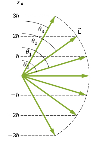
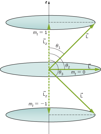
The quantization of the polar angle for the $l=3$ state is shown in (Figure). The orbital angular momentum vector lies somewhere on the surface of a cone cell with an opening angle $\theta$ relative to the z-Axis (unless $m=0,$ in which case $\theta =90\text{°}$ and the vector points are perpendicular to the z-axis).

The quantization of orbital angular momentum. Each vector lies on the surface of a cone with axis along the z-axis.

A elaborated study of cuspate impulse reveals that we cannot bon entirely three components at the same time. In the previous section, the z-component of route angular momentum has definite values that depend on the quantum number m. This implies that we cannot know both x- and y-components of triangular momentum, ${L}_{x}$ and ${L}_{y}$ , with certainty. As a result, the accurate management of the orbital angular momentum vector is unknown.

What Are the Allowed Directions? Calculate the angles that the angular momentum vector $\stackrel{\to }{L}$ can do with the z-axis for $l=1$ , every bit shown in (Figure).

The component of a given angulate impulse along the z-axis vertebra (settled away the direction of a attractive force field) can have only certain values. These are shown here for $l=1$ , for which $m=-1,0,\text{and}+1.$ The direction of $\stackrel{\to }{L}$ is quantized in the sentience that it arse make only certain angles relative to the z-axis.

Scheme The vectors $\stackrel{\to }{L}$ and ${\stackrel{\to }{L}}_{z}$ (in the z-steering) form a right triangle, where $\stackrel{\to }{L}$ is the hypotenuse and ${\stackrel{\to }{L}}_{z}$ is the adjacent side. The ratio of ${L}_{z}$ to | $\stackrel{\to }{L}$ | is the cos of the angle of interest. The magnitudes $L=|\stackrel{\to }{L}|$ and ${L}_{z}$ are given by

$L=\sqrt{l\left(l+1\right)}\hslash \phantom{\rule{0.2em}{0ex}}\text{and}\phantom{\rule{0.2em}{0ex}}{L}_{z}=m\hslash .$

Solution We are given $l=1$ , so ml can comprise $+1,0,\text{or}\phantom{\rule{0.2em}{0ex}}-1.$ Thusly, L has the value given by

$L=\sqrt{l\left(l+1\right)}\hslash =\sqrt{2}\hslash .$

The quantity ${L}_{z}$ can take three values, given by ${L}_{z}={m}_{l}\hslash$ .

${L}_{z}={m}_{l}\hslash =\left\{\begin{array}{l}\phantom{\rule{0.5em}{0ex}}\hslash ,\text{}\phantom{\rule{0.2em}{0ex}}{m}_{l}=+1\hfill \\ \phantom{\rule{0.5em}{0ex}}0,\phantom{\rule{0.5em}{0ex}}{m}_{l}=0\hfill \\ -\hslash ,{m}_{l}=-1\hfill \end{array}$

As you can see in (Figure), $\text{cos}\phantom{\rule{0.2em}{0ex}}\theta ={L}_{z}\text{/}L,$ sol for $m=+1$ , we have

$\text{cos}\phantom{\rule{0.2em}{0ex}}{\theta }_{1}=\frac{{L}_{Z}}{L}=\frac{\hslash }{\sqrt{2}\hslash }=\frac{1}{\sqrt{2}}=0.707.$

Thus,

${\theta }_{1}={\phantom{\rule{0.2em}{0ex}}\text{cos}}^{-1}0.707=45.0\text{°}.$

Similarly, for $m=0$ , we find $\text{cos}\phantom{\rule{0.2em}{0ex}}{\theta }_{2}=0;$ this gives

${\theta }_{2}={\text{cos}}^{-1}0=90.0\text{°}.$

Then for ${m}_{l}=-1$ :

$\text{cos}\phantom{\rule{0.2em}{0ex}}{\theta }_{3}=\frac{{L}_{Z}}{L}=\frac{\text{−}\hslash }{\sqrt{2}\hslash }=-\frac{1}{\sqrt{2}}=-0.707,$

so that

${\theta }_{3}={\phantom{\rule{0.2em}{0ex}}\text{cos}}^{-1}\left(-0.707\right)=135.0\text{°}.$

Significance The angles are reproducible with the figure. Exclusively the angle proportionate to the z-axis is quantized. L can detail in any direction as long as IT makes the proper lean on with the z-Axis. Frankincense, the angular impulse vectors lie on cones, as illustrated. To see how the correspondence principle holds here, consider that the smallest angle ( ${\theta }_{1}$ in the exercise) is for the maximum value of ${m}_{l},$ namely ${m}_{l}=l.$ For that smallest angle,

$\text{cos}\phantom{\rule{0.2em}{0ex}}\theta =\frac{{L}_{z}}{L}=\frac{l}{\sqrt{l\left(l+1\right)}},$

which approaches 1 as l becomes very large. If $\text{cos}\phantom{\rule{0.2em}{0ex}}\theta =1$ , so $\theta =0º$ . Moreover, for large l, there are many an values of ${m}_{l}$ , thus that all angles become possible as l gets very large.

Check Your Discernment Can the order of magnitude of ${L}_{z}$ ever be adequate L?

No. The quantum number $m=\text{−}l,\text{−}l+1\text{,…},0\text{,…},l-1,l.$ Thus, the magnitude of ${L}_{z}$ is always little than L because $<\sqrt{l\left(l+1\right)}$

Using the Wave Function to Give Predictions

As we saw earlier, we can use quantum mechanics to make predictions about physical events by the use of chance statements. It is therefore proper to state, "An electron is located within this volume with this probability at this time," but non, "An negatron is located at the position (x, y, z) at this clock time." To determine the probability of finding an electron in a hydrogen particle in a particular region of space, IT is necessary to integrate the probability density $|{\psi }_{nlm}{|}^{2}$ over that part:

$\text{Probability}={\int }_{\text{volume}}|{\psi }_{nlm}{|}^{2}dV,$

where dV is an infinitesimal volume ingredient. If this intrinsical is computed for all space, the result is 1, because the probability of the particle to be placed somewhere is 100% (the normalization condition). In a Thomas More sophisticated course on fashionable physics, you will find that $|{\psi }_{nlm}{|}^{2}={\psi }_{nlm}^{*}{\psi }_{nlm},$ where ${\psi }_{nlm}^{*}$ is the complex conjugate. This eliminates the occurrences of $i=\sqrt{-1}$ in the above figuring.

Deliberate an electron in a state of zero angular momentum ( $l=0$ ). In this case, the electron's wave operate depends only on the radial ordinate r. (Relate to the states ${\psi }_{100}$ and ${\psi }_{200}$ in (Figure).) The infinitesimal volume element corresponds to a spherical shell of wheel spoke r and infinitesimal thickness dr, graphic As

$dV=4\pi {r}^{2}dr.$

The probability of finding the negatron in the region r to $r+dr$ ("at about r") is

$P\left(r\right)dr=|{\psi }_{n00}{|}^{2}4\pi {r}^{2}dr.$

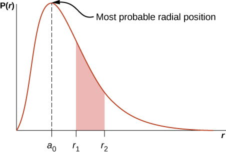
Here P(r) is named the radial probability density function (a probability per unit length). For an negatron in the ground state of atomic number 1, the probability of finding an electron in the region r to $r+dr$ is

$|{\psi }_{n00}{|}^{2}4\pi {r}^{2}dr=\left(4\text{/}{a}_{0}^{3}\right){r}^{2}\phantom{\rule{0.2em}{0ex}}\text{exp}\left(-2r\text{/}{a}_{0}\right)dr,$

where ${a}_{0}=0.5$ angstroms. The radial probability concentration function P(r) is plotted in (Figure). The area under the curve between any two radial positions, say ${r}_{1}$ and ${r}_{2}$ , gives the probability of finding the negatron in this radial range. To find the most probable radial position, we set the firstborn derivative of this go to zero ( $dP\text{/}dr=0$ ) and solve for r. The most equiprobable radial position is not equivalent to the average operating theater expectation value of the stellate posture because $|{\psi }_{n00}{|}^{2}$ is not symmetrical about its peak value.

The visible radiation chance density function for the ground state of hydrogen.

A graph of the function P of r as a function of r is shown. It is zero at r = 0, rises to a maximum at r = a sub 0, then gradually decreases and goes asymptotically to zero at large r. The maximum is at the most probable radial position. The area of the region under the curve from r sub 1 to r sub 2 is shaded.

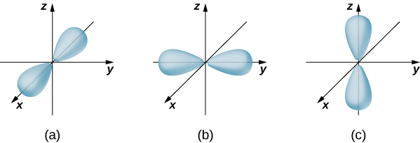
If the electron has path space impulse ( $l\ne 0$ ), and then the waving functions representing the electron depend on the angles $\theta$ and $\varphi ;$ that is, ${\psi }_{nlm}=$ ${\psi }_{nlm}$ (r, $\theta$ , $\varphi$ ). Microscopical orbitals for deuce-ac states with $n=2$ and $l=1$ are shown in (Figure). An atomic orbital is a region in space that encloses a certain percentage (ordinarily 90%) of the electron probability. (Sometimes atomic orbitals are referred to as "clouds" of probability.) Notice that these distributions are pronounced in sure directions. This directionality is important to chemists when they analyse how atoms are bound unneurotic to form molecules.

The probability density distributions for three states with $n=2$ and $l=1$ . The distributions are directed along the (a) x-Axis, (b) y-bloc, and (c) z-axis.

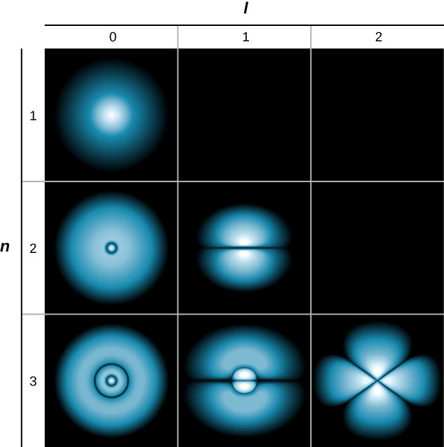
This diagram illustrates the shapes of p orbitals. The orbitals are dumbbell shaped and oriented along the x, y, and z axes.

A slightly different representation of the wave function is given in (Figure). In this case, light and dark regions point locations of relatively high and low probability, respectively. In contrast to the Niels Bohr model of the hydrogen atom, the electron does not turn the proton nucleus in a well-defined path. Indeed, the uncertainty rule makes it impossible to know how the negatron gets from unity place to another.

Probability clouds for the electron in the ground state and several worked up states of hydrogen. The chance of determination the negatron is indicated past the shade of color; the lighter the color, the greater the gamble of determination the electron.

Unofficial

A hydrogen atom commode represent described in terms of its wave function, probability density, sum up vigour, and orbital angular momentum.
The state of an electron in a hydrogen mote is specified by its quantum Numbers (n, l, m).
In contrast to the Bohr model of the atom, the Schrödinger framework makes predictions based on probability statements.
The quantum numbers of a hydrogen atom can be wont to calculate important info about the atom.

Conceptual Questions

Identify the physical implication of each of the quantum numbers of the hydrogen atom.

n (principal quantum number) $\to$ total energy
$l$ (cavity bicuspidate quantum number) $\to$ total absolute magnitude of the orbital angular impulse
m (orbital angular projection quantum number) $\to$ z-component of the orbital square impulse

Describe the ground state of hydrogen in terms of curl function, chance tightness, and atomic orbitals.

Distinguish between Bohr's and Schrödinger's mock up of the hydrogen atom. Particularly, equate the energy and route angular momentum of the ground states.

The Bohr model describes the electron as a corpuscle that moves around the proton in well-delimited orbits. Schrödinger's model describes the electron As a wave, and knowledge about the position of the negatron is restricted to probability statements. The tot up vim of the electron in the ground country (and entirely excited states) is the same for both models. However, the itinerary angular momentum of the ground state is different for these models. In Bohr's model, $L\left(\text{ground state}\right)=1$ , and in Schrödinger's model, $L\left(\text{ground state}\right)=0$ .

Problems

The wave social occasion is evaluated at rectangular coordinates ( $x,y,z$ ) $=$ (2, 1, 1) in arbitrary units. What are the spherical coordinates of this position?

$\left(r,\theta ,\varphi \right)=\left(\sqrt{6,}66\text{°},27\text{°}\right).$

If an atom has an negatron in the $n=5$ State Department with $m=3$ , what are the executable values of l?

What are the possible values of m for an electron in the $n=4$ state?

$±3,±2,±1,0$ are possible

What, if some, constraints does a appreciate of $m=1$ direct on the other quantum numbers for an electron in an atom?

What are the possible values of m for an electron in the $n=4$ state?

$±3,±2,±1,0$ are possible

(a) How many angles can L make with the z-axis for an $l=2$ electron? (b) Calculate the prise of the smallest angle.

The force connected an electron is "negative the slope of the potential energy function." Use this knowledge and (Figure) to show that the military group on the electron in a hydrogen atom is surrendered by Coulomb's force constabulary.

$F=\text{−}k\frac{Qq}{{r}^{2}}$

What is the total number of states with cavity triangular impulse $l=0$ ? (Neglect electron tailspin.)

The undulation function is evaluated at spherical coordinates $\left(r,\theta ,\varphi \right)=\left(\sqrt{3},45\text{°},45\text{°}\right),$ where the time value of the radial coordinate is inclined in arbitrary units. What are the rectangular coordinates of this position?

(1, 1, 1)

Coulomb's force law states that the ram down between two charged particles is:

$F=k\frac{Qq}{{r}^{2}}.$ Use this expression to determine the potential energy subprogram.

Study hydrogen in the earth country, ${\psi }_{100}$ . (a) Use the derivative to determine the radial berth for which the probability tightness, P(r), is a maximum.

(b) Use the integral concept to determine the norm radial position. (This is called the expectation value of the electron's radial position.) Express your answers into damage of the Bohr radius, ${a}_{o}$ . Tip: The expectation value is the honourable average esteem. (c) Why are these values different?

What is the probability that the 1s negatron of a hydrogen atom is base outside the Niels Bohr radius?

The chance that the 1s electron of a hydrogen atom is found extraneous of the Niels Bohr r is ${\int }_{{a}_{0}}^{\infty }P\left(r\right)dr\approx 0.68$

How many polar angles are possible for an electron in the $l=5$ state?

What is the level bes number of orbital angular impulse electron states in the $n=2$ shell of a hydrogen corpuscle? (Ignore negatron tailspin.)

For $n=2$ , $l=0$ (1 state), and $l=1$ (3 states). The total is 4.

What is the supreme act of orbital angular momentum electron states in the $n=3$ shell of a hydrogen atom? (Ignore electron twist.)

Glossary

bicuspid momentum orbital quantum bi (l): quantum number associated with the orbital angular momentum of an electron in a hydrogen atom

angular momentum projection quantum number (m): quantum total joint with the z-component of the orbital angular momentum of an electron in a hydrogen atom